how to draw a point mass in 3d inmatlab

Extras: Plotting in MATLAB

Contents

• Plot aesthetics
• Subplotting
• Changing the axes
• Adding text and legend
• Using the Plot Editor

One of the almost important functions in MATLAB is the plot role. The plot control also happens to exist one of the easiest functions to learn how to use. The basic syntax of the part call is shown below. This code can exist entered in the MATLAB control window or run from an m-file.

          plot(x,y)

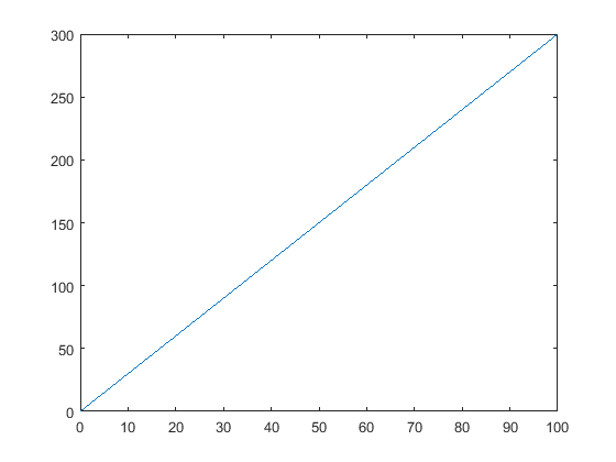
This command will plot the elements of vector y (on the vertical centrality of a effigy) versus the elements of the vector ten (on the horizontal axis of the effigy). The default is that each time the plot command is issued, the current figure volition exist erased; nosotros will discuss how to override this beneath. Consider the following unproblematic, linear function.

          y=3x

If we wished to plot this function, we could create an m-file with the following code to generate the basic plot shown below.

          x = 0:0.1:100;          y = three*10;          plot(x,y)        

Ane thing to keep in heed when using the plot control is that the vectors x and y must exist the aforementioned length. The other dimension can vary. MATLAB tin can plot a 1 x n vector versus an n x 1 vector, or a one x n vector versus a 2 x northward matrix (yous volition generate ii lines), every bit long as northward is the same for both vectors.

The plot control can also be used with just i input vector. In that case the vector columns are plotted versus their indices (the vector [1:1:north] will be used for the horizontal centrality). If the input vector contains complex numbers, MATLAB plots the real part of each element (on the horizontal axis) versus the imaginary part (on the vertical axis).

Plot aesthetics

The colour, indicate marker, and line style tin exist changed on a plot by adding a third parameter (in single quotes) to the plot command. For example, to plot the to a higher place office as a cherry-red, dotted line, change the g-file equally follows to generate the figure shown below.

          x = 0:0.1:100;           y = 3*ten;           plot(10,y,'r:')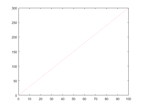        

The tertiary input consists of 1 to three characters which specify a color, betoken marker type, and/or line fashion. The list of colors, point markers, and line styles are summarized below.

          y     yellow        .     bespeak              -     solid          m     magenta       o     circle             :     dotted          c     cyan          x     x-mark             -.    dashdot          r     ruddy           +     plus               --    dashed          g     green         *     star          b     blue          south     square          west     white         d     diamond          k     black         v     triangle (down)                              ^     triangle (up)                              <     triangle (left)                              >     triangle (correct)                              p     pentagram                              h     hexagram

You can also plot more than ane function on the same figure. Allow's say you lot want to plot a sine wave and cosine moving ridge on the same set of axes, using a dissimilar color and style for each. The post-obit m-file volition plot a sine moving ridge and cosine moving ridge, with the sine wave equally a solid red line and the cosine moving ridge equally a series of green 10's.

          x = linspace(0,two*pi,50);          y = sin(x);          z = cos(ten);          plot(x,y,'r', x,z,'gx')        

By calculation more sets of parameters to plot, you can plot as many different data sets on the same figure every bit you want. When plotting many things on the same graph it is useful to differentiate the dissimilar data sets based on colour and bespeak marking. This same issue can likewise be accomplished using the hold on and hold off commands. The aforementioned plot shown above could be generated using the following lawmaking.

          x = linspace(0,2*pi,50);          y = sin(x);          plot(10,y,'r')          z = cos(x);          concord on          plot(x,z,'gx')          hold off        

E'er remember that if you employ the concur on control all plots from so on will exist generated on one ready of axes without erasing the previous plot until the hold off command is issued.

Subplotting

More than than one plot tin exist put in the same figure on its own gear up of axes using the subplot command. The subplot command allows you lot to divide the figure into equally many plots as desired, and put them all in ane figure. To use this command, the following line of code is entered into the MATLAB control window or run from an 1000-file.

          subplot(m,northward,p)

This command splits the figure into a matrix of m rows and north columns, thereby creating thousand*n plots on one figure. The p'th plot is selected as the currently active plot. For instance, suppose you want to come across a sine wave, cosine moving ridge, and tangent wave plotted on the same figure, simply not on the same axes. The post-obit code will reach this.

          10 = linspace(0,2*pi,fifty);           y = sin(x);           z = cos(10);           westward = tan(ten);            subplot(2,2,one)           plot(x,y)           subplot(ii,two,2)           plot(x,z)           subplot(2,two,three)           plot(x,w)        

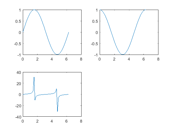
As you lot can meet, there are just three plots, even though we created a 2 ten 2 matrix of 4 subplots. We did this to show that you lot do not have to fill all of the subplots you have created, only MATLAB volition go out a spot for every position in the matrix. We could have easily made another plot using the subplot(ii,two,four) control. The subplots are arranged in the same manner as you lot would read a book. The offset subplot is in the top left corner, the next is to its right. When all the columns in that row are filled, the left-most cavalcade on the next row downward is filled (all of this is assuming that you fill up your subplots in order (i.e. ane, 2, three,...).

Ane thing to notation almost the subplot command is that every plot command issued later will place the plot in whichever subplot position was concluding used, erasing the plot that was previously in it. For example, in the thou-file above, if a plot command was issued after, it would be plotted in the third position in the subplot, erasing the tangent plot. To avert this problem, the figure should be cleared (using clf), or a new figure should exist specified (using figure).

Irresolute the axes

Now that you have found different ways to plot functions, you lot tin customize your plots. One of the virtually important ways to do this is with the axis control. The centrality command changes the centrality of the plot shown, so simply the role of the axis that is desirable is displayed. The centrality command is used by inbound the following code right after the plot command (or any command that has a plot equally an output).

          axis([xmin, xmax, ymin, ymax])

For instance, suppose want to wait at a plot of the function y=exp(5t)-1. The following lines of code will accomplish this.

          clf       t=0:0.01:5;      y=exp(v*t)-i;      plot(t,y)        

As you can see, the plot goes to infinity. Looking at the vertical axis (scale: 8e10), it is apparent that the function gets large very quickly. To get a ameliorate thought of the initial behavior of the function, allow'southward resize the axes. Enter the following control into the MATLAB command window to get a plot focused on the first 2nd of the function.

          axis([0, 1, 0, 50])        

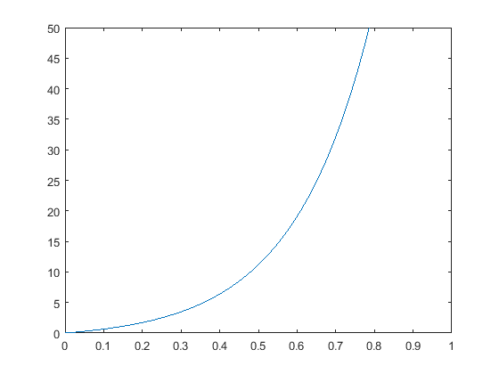
This plot may be more useful, you can now conspicuously run into what is going on as the role moves toward infinity. When using the subplot command, the axes can be changed for each subplot past issuing an axis command before the next subplot command. There are more uses of the axis command which yous can come across if y'all type help axis or doc axis in the MATLAB command window.

Calculation text and fable

Another thing that may be of import for your plots is labeling. Y'all can give your plot a championship (with the title command), x-axis label (with the xlabel command), y-axis characterization (with the ylabel control), and put text on the bodily plot. All of the above commands are issued after the actual plot command has been issued.

A title will be placed, centered, higher up the plot with the control: championship('title string'). The ten-axis label is issued with the command xlabel('x-axis string'), while the y-axis label is issued with the control ylabel('y-axis string').

Furthermore, text tin be put on the plot itself in 1 of 2 ways: the text control and the gtext command. The first command involves knowing the coordinates of where you want the text string. The syntax of the control is text(xcor,ycor,'textstring'). To utilize the other command, you do not need to know the verbal coordinates. The syntax is gtext('textstring') which provides a set of cross-hairs that yous tin can motility to the desired location with your mouse and click on the position where you want the text to be placed.

Finally, a fable can be added to the plot to identify various curves. The control is legend('string1','string2','string3'). You can specify as many text strings every bit there are curves in the plot. The default location of the legend is in the top-correct corner, but this can be modified with a parameter chosen Location.

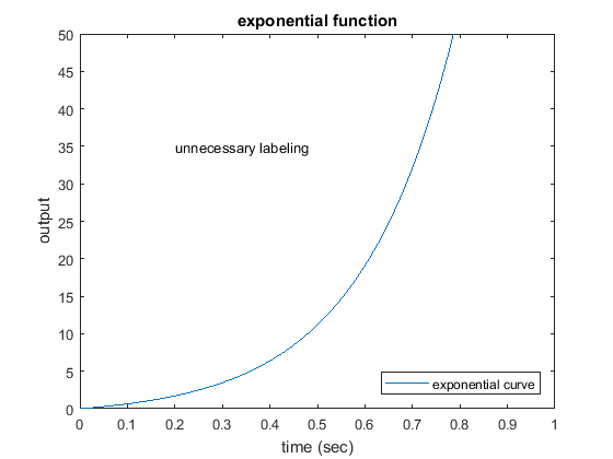
To demonstrate labeling, let's modify the exponential plot from above. Assuming that you accept already changed the axes, copying the following lines of text after the axis command will put all the labels and a legend on the plot.

          championship('exponential function')           xlabel('time (sec)')           ylabel('output')           legend('exponential curve','Location','SouthEast')           text(0.2,35,'unnecessary labeling')        

Other commands that tin exist used with the plot command are:

• figure (opens a new figure to plot on, and then the previous effigy is preserved)
• close (closes the current effigy window)
• loglog (same every bit plot, except both axes are log base 10 scale)
• semilogx (aforementioned as plot, except the x-axis is log base x scale)
• semilogy (same equally plot, except tje y-axis is log base 10 scale)
• plotyy (plots ii curves with ii axes, one on the right and one on the left)
• grid (adds grid lines to your plot)

Using the Plot Editor

In addition to entering commands in the command window to edit your plots, you can also edit plots interactively using the toolbar or drib-down menus of any figure, or past double-clicking on portions of a figure. You can specifically open the Plot Editor using the control plottools or by clicking on the icon shown below located at the right of a effigy'southward toolbar.

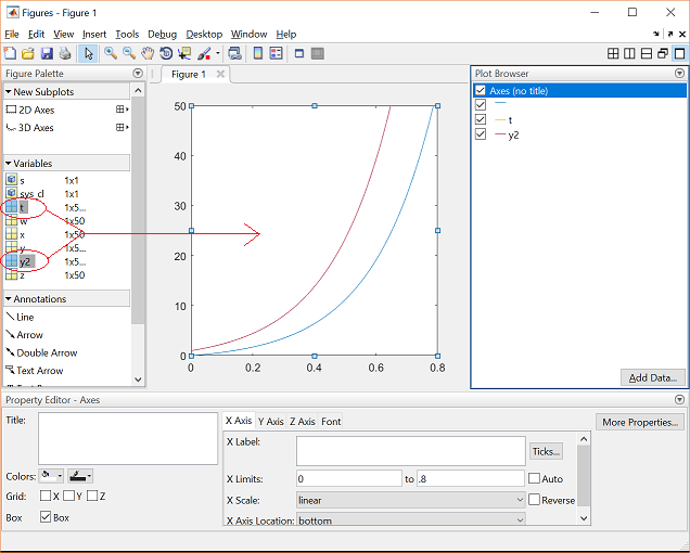
The Plot Editor consists of iii windows but i window named Figure Palette automatically opens along with the original plot the showtime fourth dimension the tool is used. Nosotros can open the other two windows named Plot Browser and Property Editor past typing the commands plotbrowser, or propertyeditor in the command window respectively. Once all windows are opened, to the left will exist the Figure Palette and to the correct volition be the Plot Browser, and at the lesser will exist the Property Editor. A picture of the Plot Editor is shown below. MATLAB volition recall the last confguration used, therefore, if any of these windows were closed in the previous session, they will non appear when the Plot Editor is opened. Typing the commands figurepalette, plotbrowser, or propertyeditor in the control window tin as well open each of these windows independently.

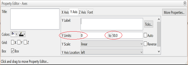
To adjust the axes of the plot for example, select the axes, and then modify the axis limits which appear in the Property Editor at the lesser of the plot.

The Holding Editor can also exist used to fix the Championship, 10 label, and Y characterization of the plot, likewise every bit the Colors and line styles of the data.

To add new data to the plot, select the x and y data from the Figure Palette in the left window (use the Ctrl cardinal to select more than than i item) and elevate them into the plot. Using y2 = 2*exp(5*t)-1;, the following plot results.

Employ the Plot Browser on the correct side of the plot to select which data should be displayed. If you have sub-plots, yous can also select or deselect which ones should exist displayed.

Of course this is non a complete account of plotting with MATLAB, but it should give you lot a nice outset.

All contents licensed under a Artistic Eatables Attribution-ShareAlike iv.0 International License.

sharpwabiagre.blogspot.com

Source: https://ctms.engin.umich.edu/CTMS/index.php?aux=Extras_Plot

Share this post